2. Download and process MODIS LAI
Phil Savoy
5/17/2021
Source:vignettes/2 Download and process MODIS LAI.Rmd
2 Download and process MODIS LAI.RmdIntroduction
This article covers downloading and processing MODIS LAI data using the StreamLightUtils package. There are a variety of sources for LAI data, but for convenience a function is included in StreamLightUtils to process two MODIS LAI products: 1.) MCD15A3H.006 which has 4 day temporal resolution and a pixel size of 500m, and 2.) MCD15A2H.006 which has 8 day temporal resolution and a pixel size of 500m. This example uses MCD15A3H but once the data has been downloaded the process is the same for either product. These products are downloaded through the AppEEARS website.
1. Submitting an AppEEARS request
The functions in StreamLightUtils are based on accessing LAI data through the AppEEARS website. This requires a NASA EARTHDATA account to access so if you do not already have an account you may register here.
To submit a request, you will need a table of basic site information. A .csv of Site_ID, Lat and Lon can be used to submit a request that extracts point samples from multiple locations.
#Make a table for the MODIS request
  request_sites <- sites[, c("Site_ID", "Lat", "Lon")]

#Export your sites as a .csv for the AppEEARS request
  write.table(
    request_sites,
    paste0(working_dir, "/NC_sites.csv"),
    sep = ",",
    row.names = FALSE,
    quote = FALSE,
    col.names = FALSE
  )
Once you have registered and exported a table of site information, you can begin by making a request:
- Click on Extract > Point Sample from the top menu bar
- On the next page select Start a new request
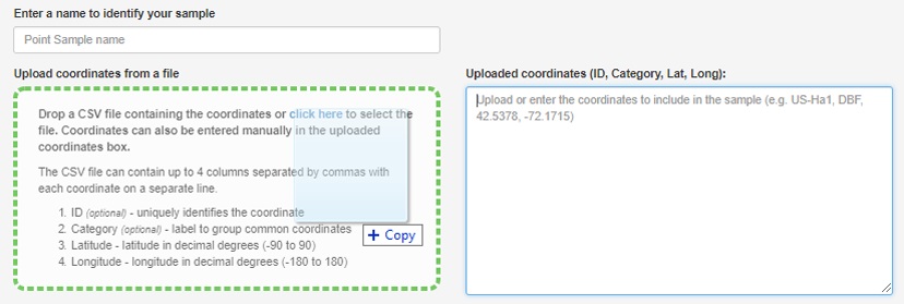
- The NC_sites.csv that was exported can now simply be drag-and-dropped to populate a list of sites. You may notice that special characters like "_" are removed from the ID field, don’t worry this is ok.
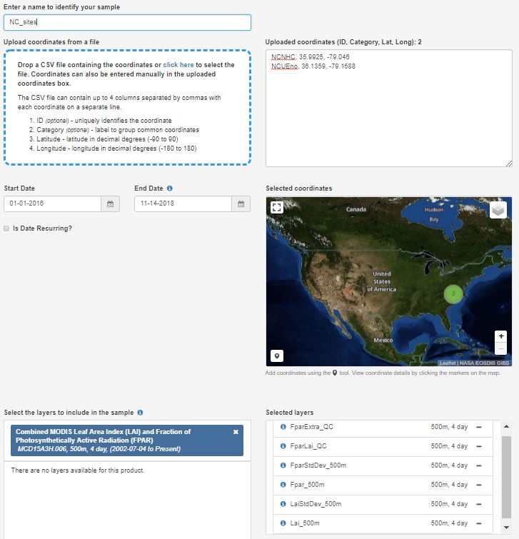
- Next, begin filling in the remaining information to submit a request including a name, Start Date, End Date, and the Selected layers.
- If possible, it is advisable to select dates with some time on either side of the desired period to estimate light. This is to help constrain some of the LAI processing steps such as interpolating to daily values. For example, if I wanted to run the model for 2015 I might download LAI data from 2014-2016.
- Type MCD15A3H into the layers search box and select the product. Add all of the layers to the selected layers.
Drag and drop site locations
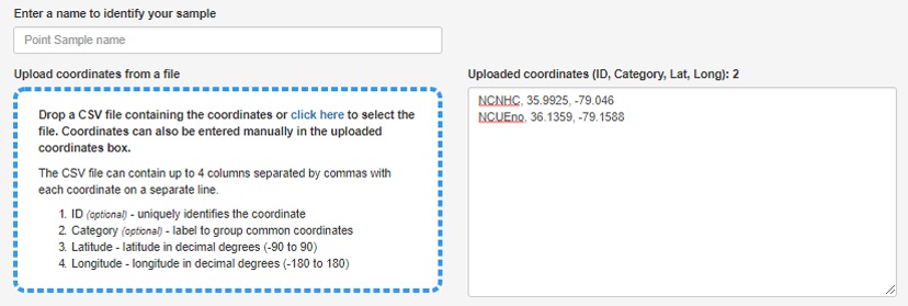
Example of request submission
Once everything is filled out submit the request. You will recieve an email notification of the request and then a second notification when the download is ready. Downloads are typically ready the same day or within a day or two depending on the size of the request. For reference, the request in this example only took 15 minutes the complete.
2. Unpacking the downloaded LAI data
Once the download is ready it can be processed using two built-in functions to StreamLightUtils. The downloaded .zip file can be unpacked using AppEEARS_unpack_QC which has the following structure:
AppEEARS_unpack_QC(zip_file, zip_dir, request_sites)
- zip_file The name of the zip file. For example, “myzip.zip”
- zip_dir The directory the zip file is located in. For example, “C:/”
- request_sites A string of site IDs
This function returns the unpacked data as a list, with each element in the list representing the data for a given site.
MOD_unpack <- AppEEARS_unpack_QC(
  zip_file = "nc-sites.zip",
  zip_dir = working_dir,
  request_sites[, "Site_ID"]
)
3. Processing the downloaded LAI data
The StreamLightUtils package leverages the phenofit package to help handling the processing of LAI data. There are a variety of curve fitting methods and this tutorial uses the approach from Gu et al. (2009) The unpacked data can then be processed using AppEEARS_proc which has the following structure:
AppEEARS_proc(Site, proc_type)
- unpacked_LAI Output from the AppEEARS_unpack_QC function
- fit_method There are several options available from the phenofit package including “AG”, “Beck”, “Elmore”, “Gu”, “Klos”, “Zhang”.
- write_ouput Logical indicating whether to write each individual driver file to disk. Default value is FALSE.
- save_dir Optional parameter when write_output = TRUE. The save directory for files to be placed in. For example, "C:/
- plot Logical, where plot = TRUE generates a plot and plot = FALSE does not
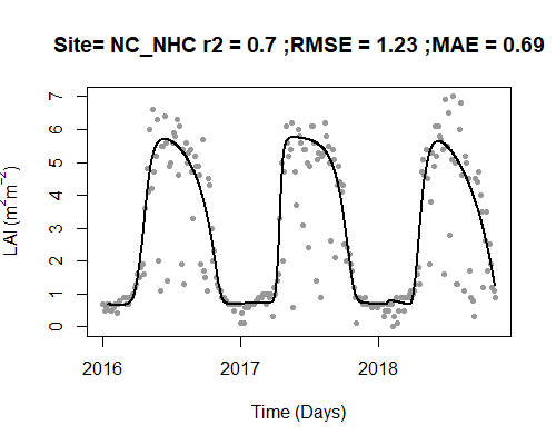
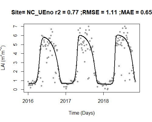
Let’s process the LAI data and visualize the results. The black line is the new fitted, interpolated, daily LAI.
MOD_processed <- AppEEARS_proc(
  unpacked_LAI = MOD_unpack,
  fit_method = "Gu",
  plot = TRUE
)